Stephen Williams

Data Transformation (T)

---

If you are looking for Extraction or Loading of Data, → Data Extraction (E)     Data Loading (L)

---

In an ETL process using Python, the transformation phase involves a series of operations to clean, restructure, and validate extracted data to prepare it for analysis or storage in a target system. Pandas library is a popular choice for these tasks due to its powerful data manipulation capabilities.

Here are 14 common data transformation techniques using Python (using simple examples):

1. Integration: Combining data from various sources (e.g., merging two dataframes based on a common key).
2. Deduplication: Removing redundant entries or duplicate rows from a dataset.
3. Aggregation: Summarizing data (e.g., calculating weekly averages from daily sales data using groupby() operations).
4. Normalization/Scaling: Standardizing numerical data to a common scale, such as scaling all values between 0 and 1, to ensure consistent data representation.
5. Imputation: Filling in missing or null values with plausible substitutes (e.g., the mean, median, or a specific value) to improve data quality.
6. Feature Engineering: Creating new, informative features from existing ones to enhance model performance (e.g., extracting month and year from a date column).
7. Filtering: Selecting a subset of data based on specific criteria or conditions.
8. Sorting: Arranging data in a specific order (ascending or descending) based on one or more columns.
9. Renaming: Changing column or index labels for clarity or consistency.
10. Pivoting/Melting: Reshaping data between "long" and "wide" formats (e.g., creating a pivot table).
11. Data Type Conversion: Changing the data type of a column (e.g., converting a string of numbers to an integer or a date string to a datetime object).
12. Encoding: Converting categorical variables into a numerical format for machine learning models (e.g., one-hot encoding or label encoding).
13. Text Cleaning/Parsing: Transforming raw text data into a usable format, including removing punctuation, converting to lowercase, or tokenization.
14. Discretization/Binning: Grouping continuous numerical data into discrete bins or intervals to simplify analysis.

let's create a sample DataFrame for demonstration:
We will be using this dataframe or part of this dataframe in the below examples.

 import pandas as pd
 import numpy as np

 data = {
    'Name': ['Alice', 'Bob', 'Charlie', 'David', 'Eve', 'Frank', 'Grace', 'Bob'],
    'City': ['New York', 'Los Angeles', 'Chicago', 'New York', 'Chicago', 'Los Angeles', 'New York', 'Los Angeles'],
    'Department': ['HR', 'Engineering', 'Engineering', 'HR', 'IT', 'Engineering', 'HR', 'Engineering'],
    'Salary': [70000, 80000, 120000, 75000, 90000, 85000, 72000, 80000],
    'Hire_Date': ['2021-01-15', '2020-03-10', '2019-06-22', '2021-04-01', '2022-09-30', '2020-11-15', '2021-07-04', '2020-03-10'],
    'Bonus_%': [5.2, np.nan, 10.1, 4.8, 8.5, 6.0, np.nan, np.nan]
 }
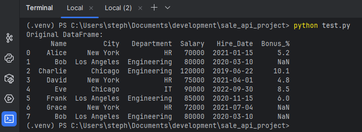
 df = pd.DataFrame(data)
 print("Original DataFrame:")
 print(df)
                    

The outcome of the above code is:

1. Integration (Merging DataFrames)

Combining two datasets based on a common key, similar to a SQL join operation.

 data2 = {'Department': ['HR', 'Engineering', 'IT'],
         'Supervisor': ['Carly', 'Guido', 'Steve']}
 df_supervisors = pd.DataFrame(data2)

 # Merge the original DataFrame with the supervisors DataFrame
 df_merged = pd.merge(df, df_supervisors, on='Department', how='left')
 print("\n1. Merged DataFrame:")
 print(df_merged)
                    

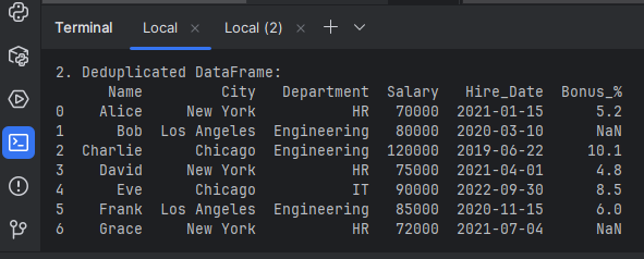
2. Deduplication

Removing duplicate rows. We have a duplicate entry for 'Bob' in 'Los Angeles'.

 # Remove exact duplicate rows, keeping the first occurrence by default
 df_deduplicated = df.drop_duplicates()
 print("\n2. Deduplicated DataFrame:")
 print(df_deduplicated)
                    

The outcome of the above code removes Name Bob and City Los Angeles as duplicate entry:

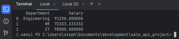
3. Aggregation

Summarizing data by grouping on one or more columns using groupby() and an aggregation function like mean(), sum(), or count().

 # Calculate the average salary per department
 df_agg = df.groupby('Department')['Salary'].mean().reset_index()
 print("\n3. Aggregated Data (Average Salary by Department):")
 print(df_agg) 
                    

The outcome of the above code is:

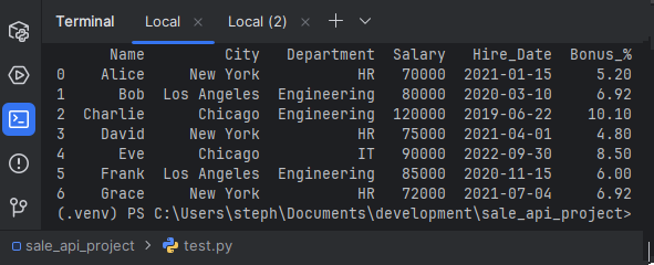
4. Imputation

Filling in missing values (NaN) in the Bonus_% column with the mean of the existing values to ensure complete data quality.

 df['Bonus_%'].fillna(df['Bonus_%'].mean(), inplace=True)
 print("\n4. DataFrame after Imputation (filled missing bonuses with mean):")
 print(df)
                

The outcome of imputing missing values of bonus (for Bob and Grace) with mean is below:

5. Feature Engineering

Creating new, useful features from existing ones. Here, extracting the hire year from the Hire_Date column.

 # Convert Hire_Date to datetime objects first
 df['Hire_Date'] = pd.to_datetime(df['Hire_Date'])
 df['Hire_Year'] = df['Hire_Date'].dt.year
 print("\n5. DataFrame after Feature Engineering (added Hire_Year):")
 print(df)
                

The outcome of adding new column Hire_Year from the current Hire_Date is below: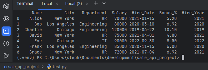

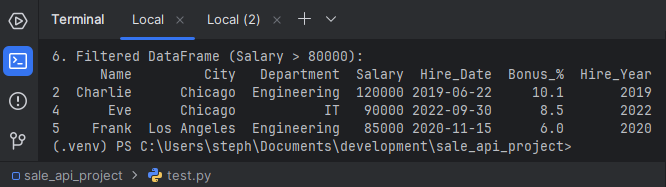
6. Filtering

Selecting a subset of data that meets specific conditions.

 # Select employees with a salary over $80,000
 df_filtered = df[df['Salary'] > 80000]
 print("\n6. Filtered DataFrame (Salary > 80000):")
 print(df_filtered)
                

The outcome of filtering employees with salary greater than 80000 is below:

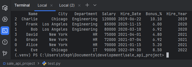
7. Sorting

Arranging data based on specific column values in ascending or descending order.

 # Sort employees by Department and then by Salary in descending order
df_sorted = df.sort_values(by=['Department', 'Salary'], ascending=[True, False])
print("\n7. Sorted DataFrame (by Department and descending Salary):")
print(df_sorted)
                

The outcome of sorting employees by Department and descending Salary is below:

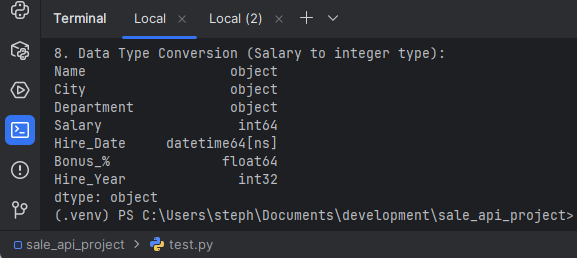
8. Data Type Conversion

Ensuring columns have the correct data types, which is essential for correct operations and memory efficiency

 # Ensure the Salary column is an integer type (although it already is in this case)
 df['Salary'] = df['Salary'].astype(int)
 print("\n8. Data Type Conversion (Salary to integer type):")
 print(df.dtypes)
                

The outcome of data type change for Salary is below:

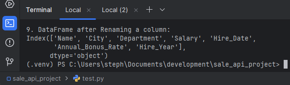
9. Renaming

Changing column names for clarity or consistency across datasets.

 df_renamed = df.rename(columns={'Bonus_%': 'Annual_Bonus_Rate'})
 print("\n9. DataFrame after Renaming a column:")
 print(df_renamed.columns)
                

The outcome of column name change for Bonus_% to Annual_Bonus_Rate is below:

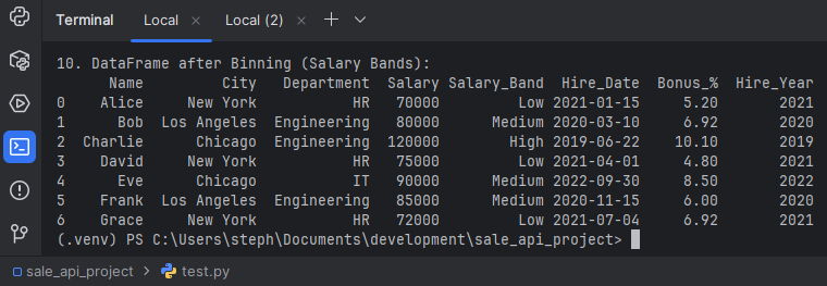
10. Discretization/Binning

Grouping continuous data into discrete bins. For example, categorizing salaries into 'Low', 'Medium', and 'High' ranges.

 bins = [60000, 75000, 90000, 130000]
 labels = ['Low', 'Medium', 'High']
 df['Salary_Band'] = pd.cut(df['Salary'], bins=bins, labels=labels)
 print("\n10. DataFrame after Binning (Salary Bands):")
 print(df[['Name', 'City', 'Department', 'Salary', 'Salary_Band', 'Hire_Date', 'Bonus_%', 'Hire_Year']])
                

The outcome of categorizing salary Annual_Bonus_Rate is below:

---

If you are looking for Data Extraction or Loading of Data, → Data Extract (E)     Data Loading (L)

---